Building a Neural Network From Scratch

by Davis Liu, Sept 2026

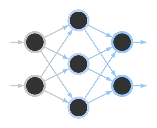
Neural networks are foundational to the most powerful implementations of machine learning. They allow computers to use existing training data to predict output for new data by discovering patterns without explicit programming.

A neural network consists of layers of neurons where the activation level of neurons in each layer are determined by the activation levels of the previous layer. Each layer of $n$ neurons can be modelled as an $n$-dimensional vector where the transitions between layers are done by applying transformations to the vector.

Modeling the Neural Network

For this analysis, we will use the row vector convention rather than the typical column vector convention used in most mathematics. So $\vec{v}T$ means apply $T$ transformation to $\vec{v}$, which is more consistent with the semantics of operators in programming and allows in place operations such as v *= M.

The easiest way to model the transition between layers is by using a linear transformation (with translation) and applying a non-linear activation function $f(x)$ to the result. The linear transformation can be done by applying the following operations in succession:

1. A matrix multiplication to represent the weights at which each neuron in the previous layer influences each neuron in the next layer
2. A linear translation by adding a vector called the bias

We can construct a network with input size $I$, output size $O$, and $n-1$ hidden layers of size $H$ (applies $n$ transformations in total). Let $a_0, \dots, a_n$ be the activation vectors for each layer, where $a_0 \in \mathbb{R}^I$ is the input vector and $a_n \in \mathbb{R}^O$ is the output vector.

We can denote the weights and biases for each layer $1 \le i \le n$ as matrix $W_i$ and vector $b_i$. Note that $W_1 \in \mathbb{R}^{I \times H}$, $\{W_2, \dots W_{n-1}\} \in \mathbb{R}^{H \times H}$, $W_n \in \mathbb{R}^{H \times O}$, $\{b_1, \dots b_{n-1}\} \in \mathbb{R}^{H}$, and $b_n \in \mathbb{R}^{O}$. Then, for every layer:

$$\vec{a}_i = f(\vec{a}_{i-1}W_i + \vec{b}_i)$$

It is also convenient to define the pre-activation vector $z_i:$

$$\vec{z}_i = f^{-1}(\vec{a}_i) = \vec{a}_{i-1}W_i + \vec{b}_i$$

Selecting the Activation Function

There are several conventional choices for the activation function, but in general, it should have the following properties:

• Non-linear: This is essential in order for the multiple layers of the network to take effect. If $f(x)$ was linear, then the transformations applied by the layers would could be simplified to a single linear transformation.
• Differentiable: This allows us to calculate gradients for the function in order to use gradient descent algorithms.
• Monotonically increasing ($\ge$): A greater weight should correspond to a greater or equal activation.

Typically, the function is one of the following (or some variant):

• Sigmoid: $f(x) = \frac{1}{1 + e^{-x}}$
  • Smooth s-shaped curve with horizontal asymptotes at $0$ (min) and $1$ (max) centered at $x = 0$.
  • This offers a good range of values constrained from $0$ to $1$, making it particularly useful for the final layer (eg. to represent probabilities).
• ReLU (Rectified Linear Unit): $f(x) = \max(0, x)$
  • Bent function (at $x = 0$) with range $0$ to $\infty$.
  • Not differentiable at $x = 0$, but this is a single point (which occurs rarely in floating point values). We can just define the derivative as $0$ (left limit) or $1$ (right limit).
  • Often yields better gradients for hidden layers because it doesn't flatten out at large values.
  • Computationally more efficient than sigmoid when range restriction isn't needed.

Training the Network — Introduction

We can train the network by initializing $W_i$ and $b_i$ with random values and running an iterative process to improve the network through multiple training steps. But first, we need to define a way to quantify how well our network is performing compared to the expected outputs. For this, we can define an error function $E(p)$, where $p$ is a vector composed of all parameters across all $W_i$ and $b_i$. In general, we define $E(p)$ as the average squared error across all training examples:

Let $T$ be the set of (input, output) pairs across all training examples. $E_{x,y}(p)$ is the error for just one example $(x,y) \in T$. Let $a_n$ be the output using the input $a_0 = x$ and the current parameters $p$.

$$ E(p) = \frac{1}{|T|} \sum_{(x, y) \in T} E_{x,y}(p) $$

$$ E_{x,y}(p) = \left|a_n - y\right|^2 $$

Then we can use a method called gradient descent to try to alter $p$ to minimize $E(p)$. Suppose there are $N$ parameters, so $p = [p_1, \dots, p_N]$. The gradient vector $\nabla E(p)$ is defined as:

$$\nabla E(p) = [\frac{\partial E(p)}{\partial p_1}, \dots, \frac{\partial E(p)}{\partial p_N}]$$

$\nabla E(p)$ points in the direction of greatest increase of $E(p)$ and its magnitude is proportional to the rate of increase. So to minimize $E(p)$, we can subtract some multiple of $\nabla E(p)$ from $p$, which we can call the learning rate $\alpha$.

Randomly Initializing the Parameters

Before we start training, we must randomly initialize the parameters. This random initialization should satisfy some properties:

• $W_i$ must be randomly initialized to avoid symmetry in the network. Otherwise, the parameters may result in similar gradient behaviour.
• The variance of $a_i$ should be roughly equal to the variance of $a_{i-1}$ to ensure a stable distribution throughout the network.
• Biases $b_i$ should generally be initialized close to $\vec{0}$.

We can analyze how to tune the random initialization so that it optimizes variance stability in a later section.

Training the Network — Computing the Gradient

To compute $\nabla E(p)$, we need to calculate $\frac{\partial E(p)}{\partial p_i}$ for every parameter $p_i$. However, that would require a lot of variables, so we can define how to take partial derivatives with respect to entire vectors $b_i$ and matrices $W_i$.

We have the following cases:

• For a scalar $y$ and vector or (flattened) matrix $x = [x_1, \dots, x_n]$, we want to define $\frac{\partial y}{\partial x}$ as $[\frac{\partial y}{\partial x_1}, \dots, \frac{\partial y}{\partial x_n}]$ to represent how each element of $x$ affects $y$.

  We can chain this derivative to a previous scalar result using scalar multiplication.

  For $f \in \mathbb{R}$:
  $(\forall i \in \{1, \dots, n\}, \frac{df}{dx_i} = \frac{df}{dy} \cdot \frac{dy}{dx_i}) \iff \frac{df}{dx} = \frac{df}{dy} \cdot \frac{dy}{dx}$.

• For a vector $y \in \mathbb{R}^n$ and vector $x \in \mathbb{R}^m$, we can define the derivative $\frac{\partial y}{\partial x}$ as a matrix $D$ such that $\partial y = \partial x \cdot D$.

  $$ [\partial y_1, \dots, \partial y_n] = [\partial x_1, \dots, \partial x_m] \cdot D \iff D = \begin{bmatrix} \frac{\partial y_1}{\partial x_1} & \dots & \frac{\partial y_n}{\partial x_1} \\ \vdots & \ddots & \vdots \\ \frac{\partial y_1}{\partial x_m} & \dots & \frac{\partial y_n}{\partial x_m} \end{bmatrix} $$

  We can chain this derivative to a previous vector or matrix result using matrix multiplication.

  For $f \in \mathbb{R} \cup \mathbb{R}^n$:
  $\frac{df}{dx} = \frac{df}{dy} \cdot D^T$.

  But in the simpler case where $D$ is a diagonal square matrix, we can flatten the result into a vector and use element-wise multiplication ($\odot$):
  $m = n \land (\forall i, j \in \{1, \dots, n\}, i \ne j \implies D_{i,j} = 0) \iff \frac{df}{dx} = \frac{df}{dy} \odot \text{diag}(D)$.

• The last case that we need to account for here is $y = a_i \in \mathbb{R}^K$ and $x = W_i \in \mathbb{R}^{J \times K}$. Formally speaking, the general derivative of a vector with respect to a matrix is a 3-D tensor consisting of every partial derivative across elements of $y$ and $x$. But this is computationally expensive.

  However, notice that $(W_i)_{j,k}$ only impacts the value of $(a_i)_k$ based on the value of $(a_{i-1})_j$ and $(b_i)_k$, so the non-diagonal tensor fields simply evaluate to $0$. We can flatten the result into a matrix $\text{diag}(D)$ that we can define as:

  $$ \begin{aligned} \text{diag}(D) &= \begin{bmatrix} (a_{i-1})_1 f'[(z_i)_1] & \dots & (a_{i-1})_1 f'[(z_i)_K] \\ \vdots & \ddots & \vdots \\ (a_{i-1})_J f'[(z_i)_1] & \dots & (a_{i-1})_J f'[(z_i)_K] \end{bmatrix} \end{aligned} $$

  We can chain this flattened derivative to a previous matrix result using element-wise multiplication ($\odot$) on corresponding element pairs whose values depend on each other.

Partial Derivative of the Biases

We will start by considering $E(p)$ for a single training example and add up errors later.

For the last layer $i = n$:

$$ \begin{aligned} \frac{\partial E(p)}{\partial b_n} &= \frac{\partial E(p)}{\partial a_n} \cdot \frac{\partial a_n}{\partial b_n} \\ &= \frac{\partial}{\partial a_n} \left[\sum_{i=1}^{O} [(a_n)_i - y_i]^2\right] \cdot \frac{\partial}{\partial b_n} f(z_n) \\ &= 2(a_n - y) \odot f'(z_n) \end{aligned} $$

For $1 \le i \lt n$:

$$ \begin{aligned} \frac{\partial E(p)}{\partial b_i} &= \frac{\partial E(p)}{\partial a_n} \cdot \frac{\partial a_n}{\partial a_i} \cdot \frac{\partial a_i}{\partial b_i} \\ &= 2(a_n - y) \cdot \frac{\partial a_n}{\partial a_i} \odot f'(z_i) \end{aligned} $$

Partial Derivative of the Weights

Define:

$$ D_{i,J,K} = \begin{bmatrix} (a_{i-1})_1 f'[(z_i)_1] & \dots & (a_{i-1})_1 f'[(z_i)_K] \\ \vdots & \ddots & \vdots \\ (a_{i-1})_J f'[(z_i)_1] & \dots & (a_{i-1})_J f'[(z_i)_K] \end{bmatrix} $$

$$ \text{copy_row}_{N}([x_1, \dots x_n]) = \begin{bmatrix} x_1 & \dots & x_n \\ \vdots & \ddots & \vdots \\ x_1 & \dots & x_n \end{bmatrix} \in \mathbb{R}^{N \times n} $$

$$ \text{copy_col}_{N}([x_1, \dots x_n]) = \begin{bmatrix} x_1 & \dots & x_1 \\ \vdots & \ddots & \vdots \\ x_n & \dots & x_n \end{bmatrix} \in \mathbb{R}^{n \times N} $$

For the last layer $i = n$:

$$ \begin{aligned} \frac{\partial E(p)}{\partial W_n} &= \frac{\partial E(p)}{\partial a_n} \cdot \frac{\partial a_n}{\partial W_n} \\ &= 2(a_n - y) \cdot \frac{\partial}{\partial W_n} f(z_n) \\ &= \text{copy_row}_{H}(2(a_n - y)) \odot D_{n, H, O} \end{aligned} $$

For $1 \lt i \lt n$:

$$ \begin{aligned} \frac{\partial E(p)}{\partial W_i} &= \frac{\partial E(p)}{\partial a_n} \cdot \frac{\partial a_n}{\partial a_i} \cdot \frac{\partial a_i}{\partial W_i} \\ &= \text{copy_row}_{H}(2(a_n - y) \cdot \frac{\partial a_n}{\partial a_i}) \odot D_{i, H, H} \end{aligned} $$

For the first layer $i = 1$:

$$ \begin{aligned} \frac{\partial E(p)}{\partial W_1} &= \frac{\partial E(p)}{\partial a_n} \cdot \frac{\partial a_n}{\partial a_1} \cdot \frac{\partial a_1}{\partial W_1} \\ &= \text{copy_row}_{I}(2(a_n - y) \cdot \frac{\partial a_n}{\partial a_1}) \odot D_{1, I, H} \end{aligned} $$

The Recursive Part

Notice that $\frac{\partial a_n}{\partial a_i}$ is shared across the derivatives for each layer and can be computed recursively.

Define:

$$ \mathcal{D}_{i,J,K} = \begin{bmatrix} (W_i)_{1,1} f'[(z_i)_1] & \dots & (W_i)_{1,K} f'[(z_i)_K] \\ \vdots & \ddots & \vdots \\ (W_i)_{J,1} f'[(z_i)_1] & \dots & (W_i)_{J,K} f'[(z_i)_K] \end{bmatrix} $$

$$ \begin{aligned} \frac{\partial a_i}{\partial a_{i-1}} &= \begin{cases} \mathcal{D}_{i, I, H} &\text{ for } i = 1 \\ \mathcal{D}_{i, H, H} &\text{ for } 1 \lt i \lt n \\ \mathcal{D}_{i, H, O} &\text{ for } i = n \end{cases} \end{aligned} $$

So we obtain the recursive formula:

$$ \begin{aligned} \frac{\partial a_n}{\partial a_n} = I_O \quad \text{(base case),} \quad \frac{\partial a_n}{\partial a_{i-1}} = \frac{\partial a_n}{\partial a_{i}} \cdot \mathcal{D}_{i,*,*}^{T} \quad \text{for } 1 \le i \le n \end{aligned} $$

Multiple Training Examples

The parts that change with each training example $(x, y)$ are:

• $y$, the target output
• $x = a_0$, the input, which impacts $a_1, \dots, a_n$

So each part involving these variables must be computed seperately for each training example.

Algorithm

Not necessarily optimized:

1. For each $(x, y) \in T$:
   1. Compute $z_0, \dots, z_n$ and $a_0, \dots, a_n$
   2. Compute $2(a_n - y)$
   3. Initialize $\frac{\partial a_n}{\partial a_i}$ to $I_O$ for $i = n$
   4. For each layer $i = n, \dots, 1$:
      1. Compute $f'(z_i)$ and $D_{i,*,*}$
      2. Put everything together to get $\frac{\partial E(p)}{\partial b_i}$ and $\frac{\partial E(p)}{\partial W_i}$ for that $(x, y)$ and store the answers in the partial gradient for $(x, y)$
      3. Multiply $\frac{\partial a_n}{\partial a_i}$ by $\mathcal{D}_{i,*,*}^{T}$ for the next iteration
   5. Multiply the partial gradient by $\frac{1}{|T|}$
2. Add all partial gradient entries to get a total gradient

Tuning the Training Parameters

Values that we must tune include the learning rate and the initial parameters.

Distributing the Initial Parameters

Previously, we stated that the variance of each layer should remain roughly stable. But it's difficult to stabilize the variance across layers in the general case, so we can normalize input to a solved case (mean of $0$, variance of $1$). We can approximate the variance of $\text{sigmoid}(x)$ as behaving like $x$ in this range and show that $\text{relu}(x)$ halves the variance of $x$. Using pre-solved variances and standard initialization techniques:

• If using $f = \text{sigmoid}$, we choose $\text{Var}(W_i) = \frac{2}{n_{\text{in}} + n_{\text{out}}}$
• If using $f = \text{relu}$, we choose $\text{Var}(W_i) = \frac{2}{n_{\text{in}}}$

Selecting the Learning Rate

Unfortunately, there isn't a mathematical formula for the optimal learning rate as it depends on the dataset. One thing that can be done is to test the rate of gradient descent (up to a limited depth) on various values (eg. $\alpha = 0.1$ to $\alpha = 10$). This can be done recursively on smaller ranges.